Predicting Bank Term Deposit Subscriptions with Machine Learning

Just now

A step-by-step journey through imbalanced data, model comparison, threshold tuning, and customer prioritisation

By Anagha C. S.

A bank can contact thousands of customers about a term deposit, yet only a small proportion will subscribe. With limited time and resources, which customers should its marketing team call first?

During my AI Residency at Apziva, I explored this question using 40,000 bank marketing records. My task was to predict subscription, identify promising customer segments, and explain which features carried useful predictive information.

After comparing 20 candidate configurations, Hist Gradient Boosting achieved 92.83% mean five-fold cross-validation accuracy. Following threshold selection, its held-out subscriber F1 was 34.60%. When I ranked customers by model score, the top 10% had a 28.25% subscription rate, compared with 7.24% overall, giving 3.90× targeting lift.

These numbers describe different aspects of the solution. The challenge was learning how to evaluate a model when most customers say no, and then connecting its predictions to an outreach decision.

Project repository: Bank Term Deposit Subscription Prediction on GitHub.

Step 1: Understand the business question.

The project focused on three questions:

• Can customer and campaign information predict whether someone will subscribe?
• Which customer segments should receive priority?
• Which features are most useful for identifying potential subscribers?

The target variable, `y`, is binary: `1` means subscribed and `0` means did not subscribe. The benchmark was at least 81% mean accuracy across five validation folds.

I defined the prediction as an action taken before a call begins. That meant the model could use only information available at that point.

Insight

The intended decision determines both the features and the evaluation. A team choosing whom to call needs subscriber precision and recall, while a team with a fixed calling budget also needs to know how well the model ranks customers.

Step 2: Set up the project and inspect the data.

Clone the repository and install its dependencies:

git clone https://github.com/Anaghacs7/ATCPCqN2T4VTrt14.git

cd ATCPCqN2T4VTrt14

pip install -r requirements.txt

jupyter notebook

Place the separately obtained project dataset at then open `notebooks/bank_subscription.ipynb`.

The excerpts below use the notebook’s function and variable names. They are checkpoints in its workflow; run the notebook in order, including its imports, configuration, cleaning, and helper definitions. Results refer to the saved notebook outputs and require the same data and compatible dependencies to reproduce.

The loading section reads the CSV, normalises column names and text values, removes accidental index columns, and explicitly maps valid target labels to 0 and 1. After that cleaning, inspect the data:

print("Shape:", bank_data.shape)

print("Exact duplicate rows:", bank_data.duplicated().sum())

display(bank_data.isna().sum())

display(bank_data["y"].value_counts())

Result

The dataset contained 40,000 records and 14 columns, with no missing values or exact duplicate rows in the recorded checks.

Inputs included age, job, marital status, education, balance, loan indicators, contact channel, campaign timing, number of contacts, and call duration.

Insight

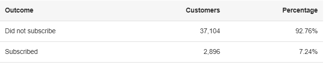
An always-no classifier would already achieve 92.76% accuracy, comfortably exceeding the project’s 81% target. The benchmark alone could therefore be met without finding a single subscriber. This made the majority baseline essential to interpreting every later result.

Step 3 : Exclude call duration and reserve the test set.

Call duration is unavailable before a call takes place. Including it could make the model appear more useful for outreach selection than it would be in practice, so I excluded it from the operational features.

customer_features = bank_data.drop(

columns=["y", "duration"], errors="ignore"

)

subscription_labels = bank_data["y"]training_customers_raw, test_customers_raw, training_labels, test_labels = (

train_test_split(

customer_features,

subscription_labels,

test_size=TEST_SIZE,

stratify=subscription_labels,

random_state=RANDOM_STATE

)

)

The notebook resets the corresponding feature and label indexes together after splitting to keep rows aligned.

Result

The stratified split produced 32,000 training records and 8,000 test records. Training data contained 2,317 subscribers; the test set contained 579.

Detailed exploration used training rows. Preprocessing and resampling were fitted inside training folds, and the test set remained separate during model and threshold selection.

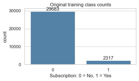
_Figure 1. Original training class counts: 29,683 non-subscribers and 2,317 subscribers. Source: the original class-count plot in the GitHub notebook._

Insight

Feature availability matters as much as predictive strength. Before deployment, campaign fields also need an availability check: a contact count, for example, must describe information known when scoring a customer, rather than include later calls.

Step 4 : Explore customer segments using rates and sample sizes

Subscriber counts and subscription rates answer different questions. A large job category may contain many buyers while having a relatively low conversion rate.

The following original code creates the counts and subscription-rate comparisons for each categorical feature:

subscribed_customers = training_eda.loc[training_eda["y"] == 1]

category_summaries = {}

for feature_name in categorical_feature_names:

summary_table = training_eda.groupby(feature_name, dropna=False, observed=True)["y"].agg(

customers="size", subscribers="sum", subscription_rate="mean"

).sort_values("subscription_rate", ascending=False)

category_summaries[feature_name] = summary_table

display(summary_table.round(4))

figure, plot_axes = plt.subplots(1, 2, figsize=(13, 4))

sns.countplot(data=subscribed_customers, y=feature_name,

order=subscribed_customers[feature_name].value_counts().index,

color="coral", ax=plot_axes[0])

plot_axes[0].set(title=f"Class 1 counts by {feature_name}", xlabel="Subscribers")

subscription_rates = summary_table["subscription_rate"].mul(100)

subscription_rates.index = subscription_rates.index.map(str)

subscription_rates.plot.barh(ax=plot_axes[1], color="steelblue")

plot_axes[1].invert_yaxis()

plot_axes[1].bar_label(plot_axes[1].containers[0], fmt="%.1f%%", padding=3)

plot_axes[1].set(title=f"Subscription rate by {feature_name}", xlabel="Subscribers (%)")

plot_axes[1].set_xlim(0, min(110, max(10, subscription_rates.max() + 10)))

plt.tight_layout()

plt.show()

It also examines numerical distributions, age groups, correlations, and statistical associations through chi-square and Mann–Whitney tests.

Result

Selected training data patterns were:

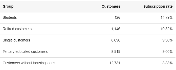
Campaign month also showed large differences. October recorded 64.62% subscriptions among just 65 training customers, while March recorded 46.76% among 216 customers.

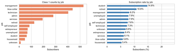
_Figure 2. Original job comparison: subscriber counts on the left and subscription rates on the right. Source: the categorical analysis in the GitHub notebook._

Insight

These patterns help generate outreach hypotheses, but sample size and campaign context affect how far they generalise. The groups overlap, so their individual rates cannot establish the rate for a combined segment. A predictive model can evaluate multiple features together, with performance checked on separate data.

Step 5: Engineer features and define preprocessing.

The notebook’s `prepare_features()` function applies fixed transformations. With `CYCLICAL_MONTH=True`, it replaces the month with sine and cosine values that represent an annual cycle:

def prepare_features(customer_data):

"""Apply fixed rules; no statistics or target information are learned here."""

engineered_features = customer_data.drop(columns=["y", "duration"], errors="ignore").copy()

if "month" in engineered_features and CYCLICAL_MONTH:

month_map = {m: i for i, m in enumerate(

["jan", "feb", "mar", "apr", "may", "jun", "jul", "aug", "sep", "oct", "nov", "dec"], 1)}

month_numbers = engineered_features["month"].astype(str).str.lower().str[:3].map(month_map)

numeric_month_values = pd.to_numeric(engineered_features["month"], errors="coerce")

month_numbers = month_numbers.fillna(numeric_month_values.where(numeric_month_values.between(1, 12)))

engineered_features["month_sin"] = np.sin(2 np.pi (month_numbers - 1) / 12)

engineered_features["month_cos"] = np.cos(2 np.pi (month_numbers - 1) / 12)

engineered_features = engineered_features.drop(columns="month")

if "pdays" in engineered_features:

days_since_previous_contact = pd.to_numeric(engineered_features["pdays"], errors="coerce")

missing_contact_time = days_since_previous_contact.isin([-1, 999])

engineered_features["pdays_sentinel"] = missing_contact_time.astype(int)

engineered_features["pdays"] = days_since_previous_contact.mask(missing_contact_time)

if "previous" in engineered_features:

previous_contact_counts = pd.to_numeric(engineered_features["previous"], errors="coerce")

engineered_features["previously_contacted"] = (previous_contact_counts > 0).astype(int)

return engineered_features

training_features = prepare_features(training_customers_raw)

test_features = prepare_features(test_customers_raw)

print("Features after engineering:", training_features.columns.tolist())

Numerical features use median imputation and standard scaling. Categorical features use most-frequent imputation and one-hot encoding, with unseen categories ignored during transformation.

numerical_column_names = training_features.select_dtypes(include="number").columns.tolist()

categorical_column_names = training_features.select_dtypes(exclude="number").columns.tolist()

numerical_preprocessing = SklearnPipeline([

("imputer", SimpleImputer(strategy="median", keep_empty_features=True)),

("scaler", StandardScaler())

])

categorical_preprocessing = SklearnPipeline([

("imputer", SimpleImputer(strategy="most_frequent", keep_empty_features=True)),

("encoder", On eHotEncoder(handle_unknown="ignore", sparse_output=False))

])

feature_preprocessor = ColumnTransformer([

("numeric", numerical_preprocessing, numerical_column_names),

("categorical", categorical_preprocessing, categorical_column_names)

])

Result

Removing duration left 12 raw predictors. Replacing month with two cyclical columns produced 13 engineered input columns; the fitted preprocessor produced 34 processed features in the saved run.

Insight

Cyclical encoding expresses the closeness of months such as December and January. Its usefulness should be compared with alternatives; the notebook can retain month for one-hot encoding instead. Scaling supports Logistic Regression and distance-based sampling experiments, while tree models generally do not require it.

Step 6: Compare models and class imbalance strategies.

The main model families were Logistic Regression, Random Forest, and Hist Gradient Boosting, alongside a majority baseline.

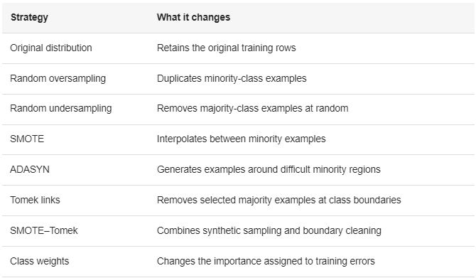
I tested original class proportions, resampling, and class weights. The reusable pipeline placed preprocessing and sampling before the classifier:

model_definitions = {

"Logistic Regression": LogisticRegression(max_iter=2000, random_state=RANDOM_STATE),

"Random Forest": RandomForestClassifier(n_estimators=160, min_samples_leaf=4,

n_jobs=-1, random_state=RANDOM_STATE),

"Hist Gradient Boosting": HistGradientBoostingClassifier(

max_iter=150, learning_rate=0.06, max_leaf_nodes=20,

l2_regularization=1.0, random_state=RANDOM_STATE)

}def build_model_pipeline(classifier, sampling_method="passthrough"):

"""Fit preprocessing, optional sampling and the classifier within each training fold."""

sampling_step = sampling_method if isinstance(sampling_method, str) else clone(sampling_method)

return ImbPipeline([

("preprocessor", clone(feature_preprocessor)),

("oversampler", sampling_step),

("model", clone(classifier))

])

Despite the step name `oversampler`, it can hold other sampling methods or pass the data through unchanged.

Result

The final comparison contained 20 candidate configurations, including three nested logistic grid searches. Some original and sampling configurations were repeated as references within the controlled sampling comparison; these were not 20 distinct algorithms.

Random oversampling balanced the training demonstration from 29,683 non-subscribers and 2,317 subscribers to 29,683 examples per class. Those demonstration arrays were not used for cross-validation.

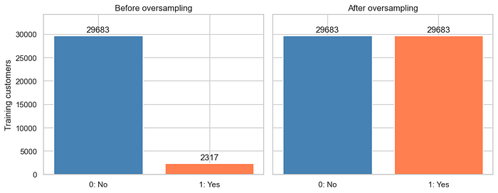
_Figure 3. The original training-only oversampling illustration. These arrays were not used for cross-validation. Source: the GitHub notebook._

Insight

Resampling must occur inside each training fold. Validation and test data retain their natural class proportions so evaluation reflects the original problem.

Get Anagha CS’s stories in your inbox

Join StartsNest for free to get updates from this writer.

Remember me for faster sign in

Synthetic methods also require care with mixed data: interpolating one-hot columns can create fractional category indicators. A categorical-aware method such as SMOTENC would be a useful future comparison with a suitable preprocessing order.

Step 7: Evaluate candidates with five validation folds.

The `evaluate_five_folds()` helper clones and fits each pipeline across five stratified folds. It returns fold metrics and out-of-fold probabilities, so each training row receives a score from a model that did not fit that row. Here is its original definition:

def evaluate_five_folds(model_pipeline, model_name, customer_features, subscription_labels):

cross_validator = StratifiedKFold(n_splits=5, shuffle=True, random_state=RANDOM_STATE)

label_array = np.asarray(subscription_labels)

fold_metric_rows = []

out_of_fold_probabilities = np.full(len(label_array), np.nan)

for fold_number, (training_indices, validation_indices) in enumerate(cross_validator.split(customer_features, label_array), start=1):

fold_model_pipeline = clone(model_pipeline)

fold_model_pipeline.fit(customer_features.iloc[training_indices], label_array[training_indices])

subscription_probabilities = predict_subscription_probabilities(fold_model_pipeline, customer_features.iloc[validation_indices])

out_of_fold_probabilities[validation_indices] = subscription_probabilities

fold_metric_rows.append({"model": model_name, "fold": fold_number,

**calculate_metrics(label_array[validation_indices], subscription_probabilities)})

return pd.DataFrame(fold_metric_rows), out_of_fold_probabilities

The full evaluation loop applies this helper to each entry in `candidate_pipelines`. It records accuracy, balanced accuracy, class-specific precision, recall and F1, ROC-AUC, and average precision.

The nested logistic searches use five outer folds and two inner folds in the executable configuration. Their inner grids examine regularization and intercept settings. The separate optional randomized search was disabled in the saved run.

Result

Selected mean validation results at threshold 0.50 were:

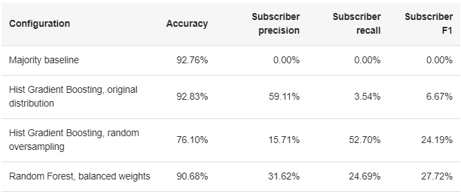
The notebook selected Hist Gradient Boosting on the original distribution by mean average precision, approximately 0.2464. Average precision summarizes performance across the precision–recall relationship and supported the customer-ranking objective.

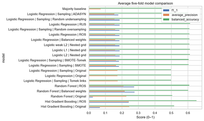
_Figure 4. Original mean five-fold comparison of subscriber F1, average precision, and balanced accuracy at threshold 0.50. Source: the GitHub notebook._

Insight

The winning configuration exceeded the accuracy target but detected only 3.54% of subscribers at the default threshold. Random Forest with balanced weights had the highest subscriber F1 at 0.50 in the saved comparison. Choosing a model therefore required an explicit objective: the notebook selected for ranking quality, then adjusted its classification threshold.

Step 8: Select a threshold using out-of-fold predictions.

A probability score can rank customers without using a single cutoff. Binary classification adds a decision threshold, which controls the trade-off between missed subscribers and unnecessary calls.

I tested thresholds from 0.01 to 0.99 using training out-of-fold scores. With `THRESHOLD_GOAL="f1"`, the notebook maximizes subscriber F1 among thresholds meeting at least 81% accuracy, using precision as a tie-breaker.

The original threshold-selection code handles both objectives and reports whether the requested constraints were met:

threshold_metric_rows = []

for threshold in np.arange(0.01, 1.00, 0.01):

threshold_metrics = calculate_metrics(training_labels, out_of_fold_probabilities_by_model[selected_model_name], threshold)

threshold_metrics["threshold"] = threshold

threshold_metric_rows.append(threshold_metrics)

threshold_results = pd.DataFrame(threshold_metric_rows)

eligible_threshold_results = threshold_results.loc[threshold_results["accuracy"] >= MIN_ACCURACY]

if THRESHOLD_GOAL == "precision":

eligible_threshold_results = eligible_threshold_results.loc[(eligible_threshold_results["precision_1"] >= TARGET_PRECISION) & (eligible_threshold_results["recall_1"] > 0)]

threshold_ranking_columns = ["recall_1", "f1_1"]

elif THRESHOLD_GOAL == "f1":

threshold_ranking_columns = ["f1_1", "precision_1"]

else:

raise ValueError("THRESHOLD_GOAL must be f1 or precision.")

threshold_constraints_met = not eligible_threshold_results.empty

if eligible_threshold_results.empty:

print("Requested constraints were not achieved. Falling back to highest training OOF F1.")

eligible_threshold_results = threshold_results

threshold_ranking_columns = ["f1_1", "precision_1"]

selected_threshold_metrics = eligible_threshold_results.sort_values(threshold_ranking_columns, ascending=False).iloc[0]

selected_threshold = float(selected_threshold_metrics["threshold"])

print("Selected threshold:", round(selected_threshold, 2))

print("Constraints met on OOF development data:", threshold_constraints_met)

display(selected_threshold_metrics.to_frame("OOF development score").round(4))

display(threshold_results.sort_values("f1_1", ascending=False).head(10).round(4))

The following notebook lines also plot the threshold trade-offs shown below.

Result

The selected threshold was 0.14. Pooled out-of-fold development results at this cutoff were:

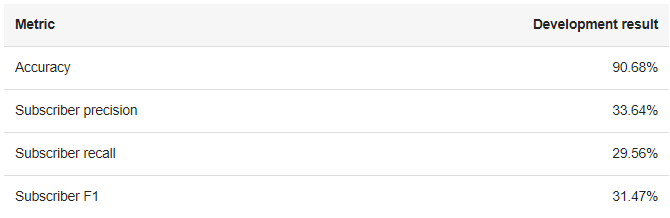
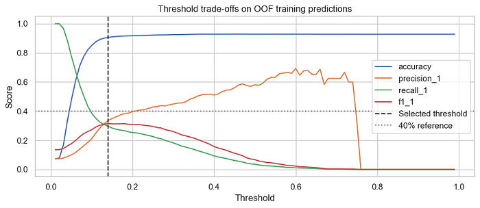
_Figure 5. Original threshold curves on development predictions, with the selected cutoff at 0.14. Source: the GitHub notebook._

Insight

Lowering the threshold recovered more subscribers. These scores were used to select the cutoff, so they are development results rather than an independent estimate of the tuned workflow. Model comparison also reuses validation data; the reserved test set provides the next evaluation after those choices are fixed.Insight

Step 9: Evaluate the final model on the test set.

The selected candidate is fitted on all training records, with any grid-search wrapper resolved to its best estimator. The following original excerpts show that fitting step and the subsequent evaluation on the untouched test data:

fitted_selected_candidate = clone(selected_model_pipeline).fit(training_features, training_labels)

final_model_pipeline = (fitted_selected_candidate.best_estimator_

if isinstance(fitted_selected_candidate, GridSearchCV)

else fitted_selected_candidate)test_probabilities = predict_subscription_probabilities(final_model_pipeline, test_features)

test_predictions = (test_probabilities >= selected_threshold).astype(int)

test_metric_scores = pd.Series(calculate_metrics(test_labels, test_probabilities, selected_threshold), name=selected_model_name)

display(test_metric_scores.round(4))

test_classification_report = classification_report(test_labels, test_predictions, labels=[0, 1],

target_names=["No (0)", "Yes (1)"], digits=4, zero_division=0)

print(test_classification_report)

Result

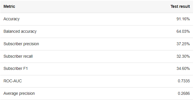
At threshold 0.14, the held-out results were:

The corresponding confusion matrix, expressed as counts, was:

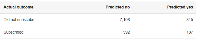
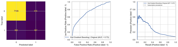
_Figure 6. Original held-out evaluation: confusion matrix at threshold 0.14, ROC curve, and precision–recall curve. Source: the GitHub notebook._

Insight

The model identified 187 of 579 subscribers, approximately one-third. Its 37.25% precision means that most customers labeled positive still did not subscribe. Neither precision nor F1 reached 40% on the test set.

Accuracy was lower than the majority baseline’s 92.76%, but that baseline found no subscribers. The model’s practical value depends on whether finding potential buyers justifies the additional calls.

Step 10: Measure customer prioritization with targeting lift.

To evaluate a fixed calling budget, I ranked all test customers by subscription score and selected the top 10%.

top_customer_count = max(1, int(np.ceil(0.10 * len(test_labels))))

top_customer_indices = np.argsort(-test_probabilities, kind="stable")[:top_customer_count]

top_subscription_rate = np.asarray(test_labels)[top_customer_indices].mean()

overall_subscription_rate = test_labels.mean()

top_lift = top_subscription_rate / overall_subscription_rate

print("Customers in top 10%:", top_customer_count)

print("Overall subscription rate:", f"{overall_subscription_rate:.2%}")

print("Top 10% subscription rate:", f"{top_subscription_rate:.2%}")

print("Top 10% lift:", round(top_lift, 2))

Result

Targeting lift = top-group subscription rate ÷ overall subscription rate ≈ 3.90×.

For comparison, a random selection of 800 customers would contain about 58 subscribers on average at the observed test prevalence. The model’s top 800 contained 226.

Insight

The ranking concentrated historical subscribers into a smaller contact list. This is retrospective targeting lift; a future campaign is needed to measure actual conversion gains and cost per subscription.

The top-decile list differs from the threshold-based list: the former contains 800 customers, while threshold 0.14 produced 502 positive predictions. Ranking supports a capacity limit; a threshold supports a binary action rule.

Step 11 Examine feature importance and individual errors

I measured permutation importance using training validation folds, with average precision as the score. The method shuffles a feature and measures the change in predictive performance.

The original code fits the model within each fold, calculates permutation importance, averages the values, and plots the result:

fold_feature_importances = []

importance_cross_validator = StratifiedKFold(5, shuffle=True, random_state=RANDOM_STATE)

for training_indices, validation_indices in importance_cross_validator.split(training_features, training_labels):

importance_model_pipeline = clone(selected_model_pipeline).fit(

training_features.iloc[training_indices], training_labels.iloc[training_indices])

permutation_results = permutation_importance(

importance_model_pipeline, training_features.iloc[validation_indices], training_labels.iloc[validation_indices],

scoring="average_precision", n_repeats=2, random_state=RANDOM_STATE, n_jobs=1)

fold_feature_importances.append(permutation_results.importances_mean)

feature_importance = pd.Series(np.mean(fold_feature_importances, axis=0), index=training_features.columns)

feature_importance = feature_importance.sort_values(ascending=False)

display(feature_importance.head(15).to_frame("mean_CV_AP_decrease"))

feature_importance.head(12).sort_values().plot.barh(figsize=(8, 4), color="steelblue")

plt.xlabel("Average precision decrease when shuffled")

plt.title("Feature importance on validation folds")

plt.tight_layout()

plt.show()

feature_importance.to_csv(RESULTS_DIRECTORY / "feature_importance.csv")

The error-analysis section uses out-of-fold training predictions to inspect false positives and missed subscribers.

Result

The leading processed inputs were `month_sin`, contact channel, day, `month_cos`, and housing-loan status. At the original-feature level, the strongest signals were campaign month, contact channel, day of month, and housing-loan status.

At threshold 0.14, exploratory out-of-fold error analysis recorded 1,632 missed subscribers and 1,351 false positives.

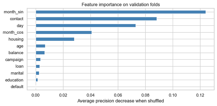
_Figure 7. Original permutation importance, measured by the mean decrease in average precision across validation folds. Source: the GitHub notebook._

Insight

Month’s two cyclical columns represent one business feature. Permutation importance shows predictive usefulness, not whether a feature increases subscriptions or causes customers to buy. Timing may capture historical campaign conditions, and related features can share importance.

These findings support investigating campaign timing and contact-channel quality, while the error counts show that subscriber detection still needs improvement. Because the threshold was selected using those out-of-fold scores, the error analysis is exploratory.

Step 12: Save the pipeline for future scoring.

The notebook saves the fitted pipeline and a JSON summary containing the selected threshold, metrics, feature names, and configuration. It also exports model comparisons, threshold results, and feature importance.

joblib.dump(final_model_pipeline, RESULTS_DIRECTORY / "subscription_pipeline.joblib")

summary_table = {

"selected_model": selected_model_name,

"threshold": selected_threshold,

"threshold_goal": THRESHOLD_GOAL,

"OOF_threshold_constraints_met": threshold_constraints_met,

"test_metrics": {metric_name: float(metric_value) for metric_name, metric_value in test_metric_scores.items()},

"top_10_percent_lift": float(top_lift),

"duration_included": False,

"cyclical_month": CYCLICAL_MONTH,

"input_features": training_features.columns.tolist(),

"top_predictive_features": feature_importance.head(5).index.tolist(),

"random_state": RANDOM_STATE

}

(RESULTS_DIRECTORY / "model_summary.json").write_text(json.dumps(summary_table, indent=2))

print("Outputs saved in:", RESULTS_DIRECTORY.resolve())

print(json.dumps(summary_table, indent=2))

Result

The saved pipeline provides a reusable scoring artifact. It expects engineered inputs, so future rows need the same cleaning and `prepare_features()` transformation before prediction.

Insight

A usable model handoff includes the threshold, input schema, feature transformations, and dependency versions. Preserving these details makes future predictions consistent with the evaluated workflow.

What I would improve next

My first priority would be validation on later campaigns. Random stratified splitting measures performance within the available historical data; a later-period test would show whether timing and channel patterns transfer. If repeated records belong to the same customer, customer identifiers would support grouped evaluation.

I would also compare categorical-aware imbalance methods, evaluate the complete model-and-threshold selection procedure within nested validation, and check calibration before treating scores as literal probabilities.

For an operational pilot, I would choose a contact cutoff around the team’s capacity, call costs, and subscription value. A prospective comparison could then measure conversion rate and cost per successful subscription.

Closing reflection

This project taught me to connect model evaluation to the decision a business needs to make. The class distribution made the accuracy target easy to exceed, while subscriber metrics exposed the harder problem. Sampling experiments showed different recall and precision trade-offs, and threshold selection made the chosen ranking model more useful for identifying potential buyers.

The final outcome was a pre-call subscription model with 34.60% held-out subscriber F1 and 3.90× top-decile targeting lift. The next step is to test that prioritization in a future campaign and establish its operational value.

This work was completed during my AI Residency at Apziva.

Notebook references

• Project repository and setup instructions
• Exploration, model comparison, threshold selection, and evaluation notebook
• My earlier article on predicting customer happiness